Machine learning for CFD — Krunal Prajapati

Why bends

Plants move solids through pipes every day: ore and sand in mining, sludge in wastewater plants, catalyst powders in chemical reactors, pulp, grain and food. The bends are where trouble starts.

At a bend, fast water is thrown against the outer wall and wears it away, while slow water on the inner side lets particles settle. The turn also sets the water swirling sideways in two vortices, called Dean vortices, which decide where the particles go. We chose a bend to study them.

Cross-section, 1 D after the bendLooking down the pipe, outer wall at the top. The lines follow the sideways flow: two counter-rotating swirls.

Mining slurries
Wastewater
Chemical reactors
Pulp and paper
Food and grain

The thesis run at t = 2.00 s, cut open along the pipe’s mid-plane: blue is slow, red is fast. Drawn to scale from the dataset.

Problem

To see inside a pipe like this, engineers use computational fluid dynamics (CFD). The software splits the pipe into a mesh of tiny cells and solves the equations of fluid motion in every one, in small steps through time.

It is accurate, but slow, and every change to the setup means running it again. In the semester before this thesis I ran these simulations in OpenFOAM and waited on them. This thesis asks whether a model trained on the first part of a run can predict the rest, faster than the solver.

Probe tip and the current snapshotPipe sample, stand, readout and slide rackMesh points on the cut faceReal data from the thesis run. The cut face is the plane one diameter after the bend, coloured by water speed, with its 553 mesh points. The probe sits on one point, and the box shows that point’s velocity and pressure at the current snapshot. Slides left of the stop block (up to 1.5 s) trained the model; the rest tested it.

20×

less compute time for the trained model than for the solver

saved time steps, every 0.05 s from 0 to 2 s

135,730

rows in each saved step, one per mesh point

sample planes, one before the bend and three after it

Case

A 40 mm pipe with a 90° bend, set up from OpenFOAM’s bentPipe example. Water enters at 0.5 m/s, about walking pace, carrying solid particles that make up 0.1% of its volume. It runs 10 diameters, turns upward and runs 10 more.

Solver: multiphaseEulerFoam, OpenFOAM 10
Phases: Water and particles, each treated as a fluid that fills the pipe (Euler–Euler)
Pipe: 40 mm diameter, 60 mm bend radius (1.5 D), 10 D straight on each side
Inlet: Water at 0.5 m/s, particles at 0.1% by volume
Outlet: 1 bar
Walls: Water sticks to the wall, particles slide along it. Turbulence near the wall uses the k-ε model.
Density ratio: 1.4: particles are 40% heavier than the same volume of water
Temperature: Constant (isothermal)
Reynolds number: About 20,000: turbulent, full of small eddies

Drawn to scale from the mesh. Hover a sample plane to find it in the drawing.

Particles

The particles are split into 30 size classes from 1 to 250 µm, spaced evenly on a log scale. The solver tracks how much particle volume sits in each class as particles collide, stick together and break apart.

Circle sizes follow the log scale, not true size: the largest class is 250 times the width of the smallest. Shares are of the particle volume at the inlet, from the size distribution below.

Physics

The solver doesn’t follow each grain. It treats the particles as a second fluid mixed through the water, with its own speed at every point. Four forces pass momentum between the two.

Drag uses the Wen–Yu model and lift the Saffman–Mei model. Gravity also acts: the particles are 1.4 times as dense as water.

The equationsOptional

\frac{\partial (α_{φ} ρ_{φ})}{\partial t} + \nabla \cdot (α_{φ} ρ_{φ} u_{φ}) = 0

Mass. Nothing appears or disappears. For each phase φ: volume fraction α, density ρ, velocity u.

\frac{\partial (α_{φ} ρ_{φ} u_{φ})}{\partial t} + \nabla \cdot (α_{φ} ρ_{φ} u_{φ} u_{φ}) - \nabla \cdot (α_{φ} τ_{φ}) = - α_{φ} \nabla p + α_{φ} ρ_{φ} g + M_{φ} + S_{φ}

Momentum. Newton’s second law for a fluid: stress τ, pressure p, gravity g, exchange M with the other phase, source S.

M_{φ} = \sum_{ψ \neq φ} (F_{D} + F_{L} + F_{TD} + F_{VM})

Exchange. The four forces above: drag, lift, turbulent dispersion and virtual mass.

Sticking and breaking

On the way through the pipe, particles bump into each other. Some stick and grow (aggregation). Strong eddies tear others apart (breakage). The solver tracks both, moving particle volume between the size classes.

How often each happens depends on particle size and on how turbulent the water is. The two charts show the rules the solver uses.

The equationsOptional

\frac{\partial n (v)}{\partial t} + \nabla \cdot (u n (v)) = S_{v}

Population balance. Counts particles of each volume v as they move, stick and break. S_v holds aggregation and breakage.

a_{d, d^{'}} = \frac{4}{3} \sqrt{\frac{3 π}{10}} \sqrt{\frac{ε}{ν}} {(d + d^{'})}^{3}

Aggregation. Adachi et al. (1994). ε: how fast turbulence burns energy, ν: kinematic viscosity.

b_{v^{'}} = \sqrt{\frac{4}{15 π}} \sqrt{\frac{ε}{ν}} \exp (- \frac{ε_{cr}}{ε})

Breakage. Kusters (1991). ε_cr = B / r_c, from particle strength B and collision radius r_c.

Sticking rate for every pair of sizes

1 µm10100250 µm

Hover a cell.

Breaking rate against turbulence

Hover the curve.

Left: darker means two particles of those sizes stick more often, relative to two 1 µm particles. Large pairs stick millions of times more often. Right: below a critical turbulence level (ε_cr) particles barely break; above it, breakage climbs toward its limit.

Size distribution

Read it like a histogram: the higher a curve, the more particle volume sits at that size. At the inlet the peak is around 25 µm. One diameter after the bend it has moved to about 55 µm, and by nine diameters it is near 66 µm, as particles stick together on the way up the pipe.

Fig. 4.1 from the thesis, digitised: the volumetric density in each of the 30 classes at one time step.

Simulation

What the 41 saved steps show, read straight from the dataset.

Flow

Blue is slow and red is fast. The water starts at 0.5 m/s everywhere. Water touching a wall can’t move, so over the first second a slow layer grows from the walls, and the bend throws the fastest water toward its outer wall. From about 1.4 s on, the field barely changes.

Below, the pipe’s mid-plane is straightened out with the inlet on the left, and the four sample planes sit under it. Arrows on the planes show the sideways flow.

Inner wall of the bendt = 0.05 s

Outer wall of the bendInlet on the left, outlet on the right

Water speed |U|00.350.70 m/s

Planes seen from downstream, outer wall at the top

|U| on the x = 0 plane and on the four sample planes at all 41 saved times. The strip is stretched four times across the pipe so the walls stay readable. Hover anywhere for the value.

Dean vortices

This swirl is why we picked a bend. In the bend, the fast water in the middle of the pipe is flung toward the outer wall, the way you lean outward in a turning car. The slow water near the walls can’t keep up, so it is pushed back around the sides toward the inner wall. The result is two counter-rotating swirls, named after W. R. Dean, who described them in 1927.

A stirred cup of tea does the same thing: the leaves gather in the middle of the bottom because a sideways circulation sweeps them there.

Collar: where the cross-section is takenPipe, supports, rail and viewerStreamlines of the sideways flowReal data at t = 2.00 s. The collar rides a rail up the vertical leg, ticked every half diameter from the bend’s exit. The screen shows the cross-section at the collar, outer wall at the top, coloured by water speed, with streamlines of the sideways flow traced from the dataset: two counter-rotating swirls. The dial reads the fastest sideways flow there, up to 0.25 m/s.

0.25m/s

peak sideways flow, inside the bend: half the speed the water enters with

11,500

Dean number. Above about 100 the swirls are strong; this flow is far past that.

0.05m/s

still swirling ten diameters after the bend: a tenth of the inlet speed

Hover the chart.

Every mesh section along the pipe at t = 2.00 s. The swirl starts inside the bend, peaks just before its exit and fades slowly up the vertical leg. The coloured ticks are the thesis sample planes.

Profiles

Speed across the pipe, from the bend’s inner wall to its outer wall. Before the bend the profile is flat and symmetric. One diameter after it, the outer half runs at about 0.61 m/s while the inner half drops to about 0.33 m/s.

On the bend plane (x = 0) of each sample plane. The time control is shared with the flow figure above.

Model

From 41 CSV files to two XGBoost models.

How it works

From the solver’s output to a prediction, in six steps. Every number in this walkthrough comes from the thesis run.

Simulate

OpenFOAM solves the flow and saves a snapshot every 0.05 s: 41 from 0 to 2 s. Here is one cross-section, one diameter after the bend, in 14 of them. Watch the slow region grow.

Export

ParaView exports each snapshot as a table, one row per mesh point: where it is, and the water’s velocity and pressure there. Five of this plane’s points are picked out.

Follow a point

Line the 41 tables up by point ID, and every point gets a history: how its velocity changed over the run. This is one point, 7 mm off the centre line.

Build rows

Slide along the history. At each step, the point’s last three values of Ux and its current Uy and Uz are the inputs, and its current Ux is the answer to learn. Every point at every step gives one row.

Train

Rows from the first 1.5 s train XGBoost, which learns how the inputs map to the answer one small decision tree at a time. One model is trained for each velocity component.

Predict

For the steps after 1.5 s the model predicts the velocity at every point. Its fields are then drawn next to the solver’s to see how close they come.

1 / 6

Dataset

I exported the run from ParaView as one CSV per saved time step: 41 files, 651 MB in all. Each row is a mesh point with its position, the water’s velocity and the pressure. The files went to Kaggle for training.

Point ID	Points_0	Points_1	Points_2	U.water_0	U.water_1	U.water_2	\|U\|	p	p_rgh
112898	-0.001866	0.456234	0.100000	-0.015046	0.143468	0.326067	0.356552	103556.0	104534.5
112899	0.000000	0.456222	0.100000	0.000000	0.161616	0.311972	0.351349	103556.5	104535.0
112900	0.001866	0.456234	0.100000	0.015047	0.143467	0.326067	0.356551	103556.0	104534.5
112909	-0.001885	0.458115	0.100000	-0.019699	0.118715	0.308863	0.331478	103558.0	104536.5
112910	0.000000	0.458109	0.100000	0.000000	0.133207	0.298873	0.327214	103558.5	104537.0
… 135,725 more rows in this file, and 40 more files

Five rows from t1.55.csv, on the 1D-after plane. Positions in metres, velocity in m/s, pressure in Pa. The same files build every flow figure on this page.

Train and test

The model trains on every saved step up to 1.5 s and predicts the next ten, from 1.55 to 2.0 s. Most of the change in the flow happens before 1.4 s, so the test window is the flow settling into its final state.

Peak |U| on each sample plane at every saved step. The 1D-after plane speeds up as the jet along the outer wall forms. The 5D plane overshoots near 0.8 s before settling.

Features

One model per velocity component. To predict Ux at a point, the model gets Uy and Uz at that time and Ux at the three steps before. The water’s volume fraction can be added as an optional feature.

Target

Real values in m/s from one mesh point on each sample plane, 7.4 mm off the symmetry plane. Each row is one training example.

XGBoost

XGBoost builds an ensemble of small decision trees. Each new tree fits what the trees before it got wrong, and its output is added with a small weight.

Trees

A gradient-boosted model fitted live in your browser to one real profile, 1D after the bend at t = 1.55 s: depth-2 trees, learning rate 0.3. The thesis models work the same way on many more features and points.

Accuracy

Strong results on tabular regression with little tuning.

Non-linear

Trees capture sharp changes, like the jump at the edge of the slow region.

Regularisation

Penalties on tree size and leaf weights hold back overfitting.

Feature importance

Shows which inputs the predictions lean on.

Scale

Trains on millions of rows on a laptop or a Kaggle notebook.

Robust

Copes with sparse and unscaled inputs.

Learning rate, tree depth and the number of trees were chosen by grid search, with an 80/20 train–validation split and cross-validation. Scored with mean squared error, mean absolute error and R².

Results

How close the predictions came, and how fast.

Size predictions

The first model predicted the volumetric density in each size class over time, on each sample plane. Before the bend the two curves overlap. Further downstream the model overshoots the peak, and the error grows.

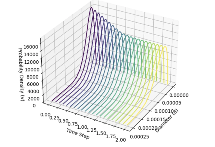
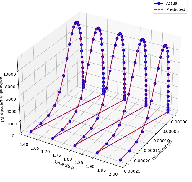
CFD volumetric density against diameter for every saved time step, 1D before the bend — CFD: the distribution at every saved step, 0 to 2 s

Predicted and actual volumetric density over the test steps, 1D before the bend — CFD: the distribution at every saved step, 0 to 2 s

Fig. 4.2 and 4.3 from the thesis.

Mean squared error by plane

Table 4.1. Log scale: each grid step is ten times the last. Error rises about 400 times from before the bend to nine diameters after it.

Velocity predictions

The second model predicted the water’s velocity at every point on the sample planes. At 1.55 and 1.60 s the predicted fields keep the shapes of the CFD result, including the slow region on the inner wall after the bend.

Water speed |U|00.350.70 m/s

Both fields are read back from the colours of the thesis figures. Checked against the CFD export, the decoded CFD fields are within 0.003 m/s on average, so the gap shown here is the model’s. The bands in the gap view are the contour levels of the original plots.

Accuracy

Errors per velocity component, over all test points. Uz, the flow direction up the vertical leg, has the largest: a mean absolute error of 0.054 m/s, about a tenth of the inlet speed.

Mean squared error

Mean absolute error

Table 4.2. MSE in m²/s², MAE in m/s.

Speed

Once trained, the model produced its predictions with about 20 times less compute time than the solver run it stands in for.

CFD solver

1×

XGBoost

1/20

The same job, drawn to the thesis’ 20× figure: each bar fills in the time its method takes.

Next steps

What the thesis left for later.

Physics-informed models

Build the governing equations into the model, so predictions respect mass and momentum and hold up on new flow conditions.

Hybrid ML and CFD

Let the model explore a design space quickly, or give the solver a starting guess, and keep the solver for the final answer.

Real-time use

Fast predictions could feed flow control, monitoring and predictive maintenance in plants.

Other geometries

The same method applies to branching pipes, porous media and fluidised beds.

Uncertainty

Report how confident each prediction is, which matters where a wrong answer is costly.

This thesis is where I first ran into how hard OpenFOAM is to set up. A few years later I built OpenFOAM Studio, a desktop app that writes and runs OpenFOAM cases from plain English.

OpenFOAM Studio →

References

Dutta, Saha, Nandi and Pal. Numerical study on flow separation in 90° pipe bend under high Reynolds number by k-ε modelling. Engineering Science and Technology, 2016.
Kim, Yadav and Kim. Characteristics of secondary flow induced by 90-degree elbow in turbulent pipe flow. Engineering Applications of CFD, 2014.
Xu et al. Bent pipe flow reconstruction based on improved ultrasound Doppler velocimetry and radial basis function neural network. Flow Measurement and Instrumentation, 2023.
Cao, Xu and Jiang. Physics-informed machine learning based RANS turbulence modeling of convection heat transfer of supercritical pressure fluid. Int. J. Heat and Mass Transfer, 2023.
Duraisamy. Perspectives on machine learning-augmented Reynolds-averaged and large eddy simulation models of turbulence. Physical Review Fluids, 2021.
Font, Weymouth, Nguyen and Tutty. Deep learning of the spanwise-averaged Navier–Stokes equations. Journal of Computational Physics, 2021.
Sharma, Chung, Akoush and Ihme. A review of physics-informed machine learning in fluid mechanics, 2023.
Wang, Ding and Shao. The improved radial basis function neural network and its application. Artificial Life and Robotics, 1998.